Processing a wavefront metrology experiment#
Converting raw data at the Sigray lab#
Attention
The file structure is written for the experiments at the Sigray lab only.
Here we wrote a small auxiliary snippet of code, that defines the paths to image and
log files. We’ll need them to generate a pyrost.STData container:
>>> import pyrost as rst
>>> import os
>>> scan_num = 2989
>>> log_path = f'/gpfs/cfel/group/cxi/labs/MLL-Sigray/scan-logs/Scan_{scan_num:d}.log'
>>> data_dir = f'/gpfs/cfel/group/cxi/labs/MLL-Sigray/scan-frames/Scan_{scan_num:d}'
>>> data_files = sorted([os.path.join(data_dir, path) for path in os.listdir(data_dir)
>>>                      if path.endswith('Lambda.nxs')])
>>> wl_dict = {'Mo': 7.092917530503447e-11,
>>>            'Cu': 1.5498024804150033e-10,
>>>            'Rh': 6.137831605603974e-11}
Now we need to read a log file to generate a set of basis vectors and sample translations.
We use pyrost.KamzikConverter Kamzik log files converter, which provides an interface
to read log files with pyrost.KamzikConverter.read_logs():
>>> converter = rst.KamzikConverter()
>>> converter = converter.read_logs(log_path)
After the data is obtained from the log files, it’s written to converter.log_attr and
converter.log_data attributes. As next, one can get a list of datasets available in log
data with pyrost.KamzikConverter.cxi_keys() method:
>>> converter.cxi_keys()
['basis_vectors', 'dist_down', 'dist_up', 'sim_translations', 'log_translations']
Here, ‘basis_vectors’ is a set of basis vectors, ‘dist_up’ and ‘dist_down’ are up-lens-to-detector and down-lens-to-detector distances respectively, and ‘sim_translations’ and ‘log_translations’ are a set of sample translations read from log files and simulated based on log attributes. In our case, we would like to get a set of basis vectors (‘basis_vectors’) and sample translations (‘log_translations’):
>>> log_data = converter.cxi_get(['basis_vectors', 'log_translations'])
Now we’re ready to generate a pyrost.STData container. It requires a data file with X-ray images,
that can be opened with pyrost.CXIStore file handler, also we parse attributes obtained from log
files (log_data) and some extra information obtained from the experimental setup:
>>> input_file = rst.CXIStore(data_files)
>>> data = rst.STData(input_file, **log_data, distance=2.0, wavelength=wl_dict['Mo'])
Now we can inspect what attributes are already stored inside of container:
>>> data.contents()
['y_pixel_size', 'distance', 'translations', 'basis_vectors', 'x_pixel_size',
'good_frames', 'wavelength', 'num_threads', 'input_file']
pyrost.STData is the main class, that provides different tools to process the data. Also, it provides
methods to load data from a file with pyrost.STData.load() and save to it with pyrost.STData.save().
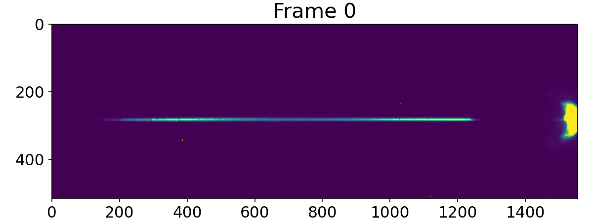
Let’s load raw X-ray images and look at them:
>>> data = data.load('data')

>>> fig, ax = plt.subplots(figsize=(8, 3))
>>> ax.imshow(data.data[0], vmax=100)
>>> ax.set_title('Frame 0', fontsize=20)
>>> ax.tick_params(labelsize=15)
>>> plt.show()
Note
We may save the data container to a CXI file at any time with pyrost.STData.save()
method, see the section Saving the results in the Diatom dataset tutorial.
Working with the data#
The function returns a pyrost.STData data container, which has a set of utility routines
(see pyrost.STData for the full list of methods). Usually, the pre-processing of a Sigray
dataset consists of (see Preprocessing of a PXST dataset for more info):
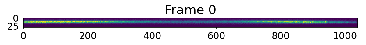
Defining a region of interest [y_min, y_max, x_min, x_max] (
pyrost.Crop,pyrost.STData.update_transform()).Mirroring the data around the vertical detector axis if needed (
pyrost.Mirror,pyrost.STData.update_transform()).Masking bad pixels (
pyrost.STData.update_mask()).
>>> crop = rst.Crop([270, 300, 200, 1240])
>>> mirror = rst.Mirror(axis=1, shape=(crop.roi[1] - crop.roi[0], crop.roi[3] - crop.roi[2]))
>>> transform = rst.ComposeTransforms([crop, mirror])
>>> data = data.update_transform(transform=transform)
>>> data = data.update_mask(vmax=100000)
>>> fig, ax = plt.subplots(figsize=(8, 3))
>>> ax.imshow(data.data[0], vmax=100)
>>> ax.set_title('Frame 0', fontsize=20)
>>> ax.tick_params(labelsize=15)
>>> plt.show()
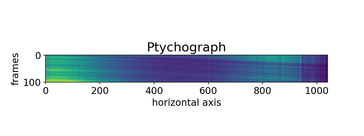
Integrating the stack of frames along the vertical detector axis (
pyrost.STData.integrate_data()).
>>> data = data.integrate_data()
>>> fig, ax = plt.subplots(figsize=(8, 3))
>>> ax.imshow(data.data[:, 0])
>>> ax.set_title('Ptychograph', fontsize=20)
>>> ax.set_xlabel('horizontal axis', fontsize=15)
>>> ax.set_ylabel('frames', fontsize=15)
>>> ax.tick_params(labelsize=15)
>>> plt.show()
Estimating the focus-to-sample distance (
pyrost.STData.defocus_sweep(),pyrost.STData.update_defocus()).
>>> defoci = np.linspace(50e-6, 300e-6, 50)
>>> sweep_scan = data.defocus_sweep(defoci, size=50)
>>> defocus = defoci[np.argmax(sweep_scan)]
>>> print(defocus)
0.00015204081632653058

>>> fig, ax = plt.subplots(figsize=(8, 4))
>>> ax.plot(defoci * 1e3, sweep_scan)
>>> ax.set_xlabel('Defocus distance, [mm]', fontsize=15)
>>> ax.set_title('Average gradient magnitude squared', fontsize=20)
>>> ax.tick_params(labelsize=15)
>>> ax.grid(True)
>>> plt.show()
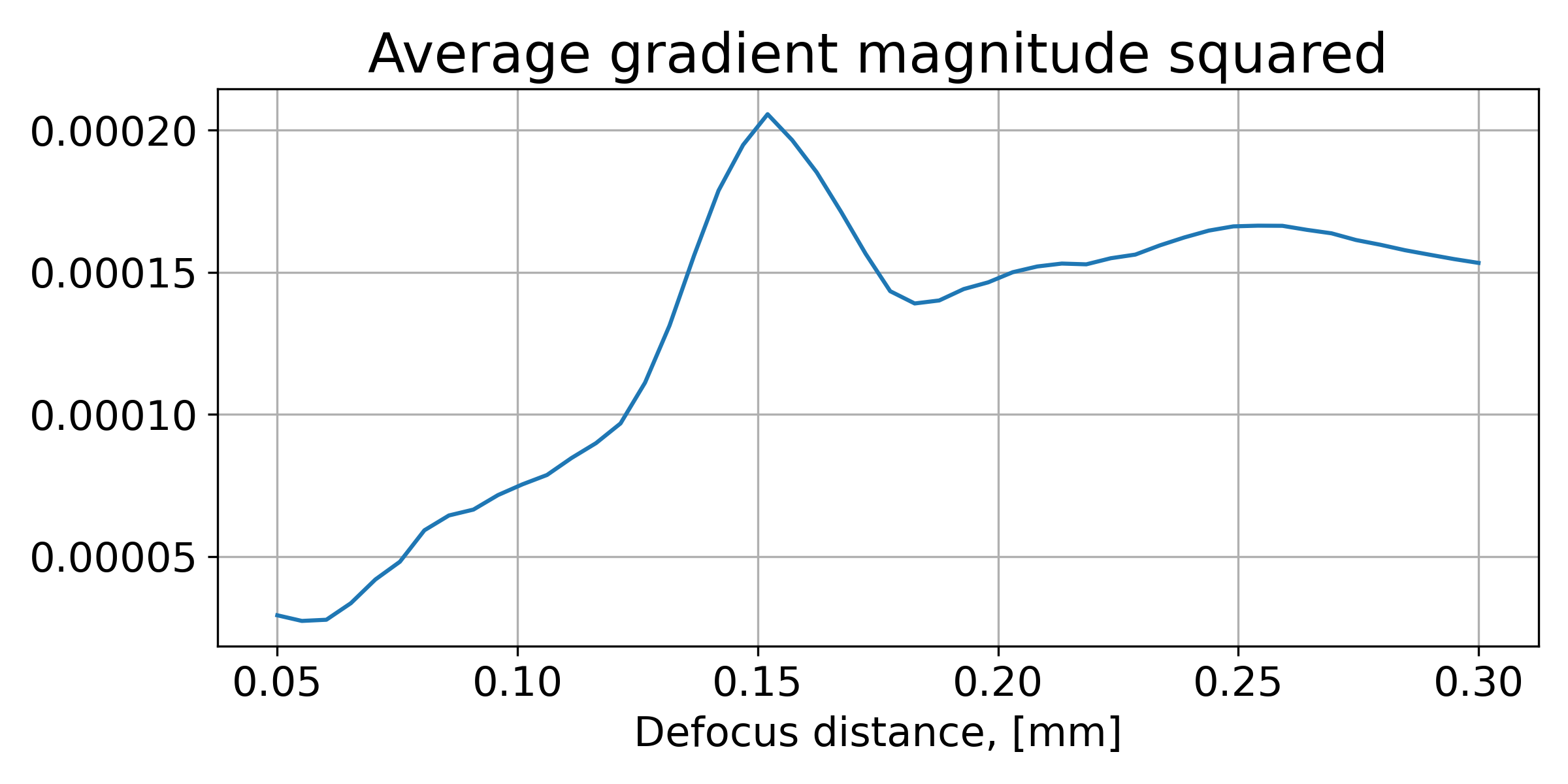
Let’s update the data container with the defocus distance we got.
>>> data = data.update_defocus(defocus)
Speckle tracking update#
The steps to perform the speckle tracking update are also the same as in Speckle tracking update:
Create a
pyrost.SpeckleTrackingobject.Find an optimal kernel bandwidth with
pyrost.SpeckleTracking.find_hopt().Perform the iterative R-PXST update with
pyrost.SpeckleTracking.train()orpyrost.SpeckleTracking.train_adapt().
>>> st_obj = data.get_st()
>>> h0 = st_obj.find_hopt()
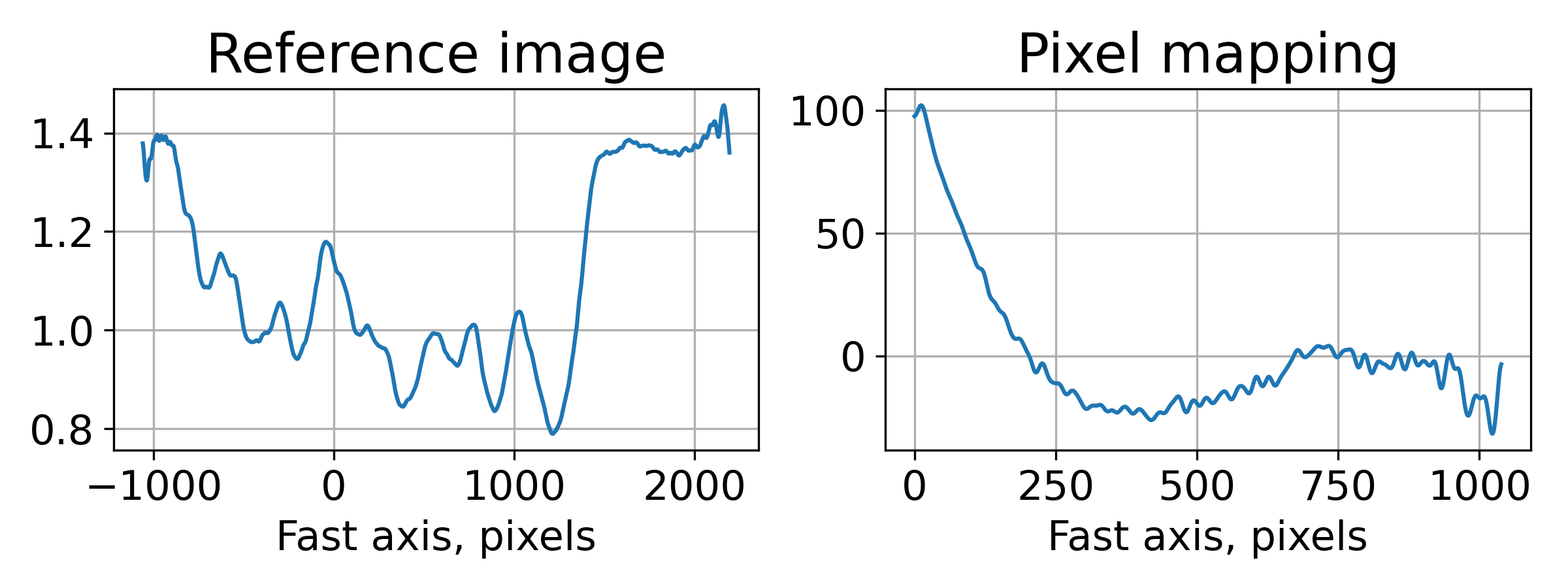
>>> st_res = st_obj.train_adapt(search_window=(0.0, 10.0, 0.1), h0=h0, blur=8.0)
>>> fig, axes = plt.subplots(1, 2, figsize=(8, 3))
>>> axes[0].plot(np.arange(st_res.reference_image.shape[1]) - st_res.ref_orig[1],
>>> st_res.reference_image[0])
>>> axes[0].set_title('Reference image', fontsize=20)
>>> axes[1].plot((st_res.pixel_map - st_obj.pixel_map)[1, 0])
>>> axes[1].set_title('Pixel mapping', fontsize=20)
>>> for ax in axes:
>>> ax.tick_params(labelsize=10)
>>> ax.set_xlabel('Fast axis, pixels', fontsize=15)
>>> ax.grid(True)
>>> plt.show()
After we successfully reconstructed the wavefront with pyrost.SpeckleTracking.train_adapt()
we are able to update the pyrost.STData container with pyrost.STData.import_st()
method.
>>> data.import_st(st_res)
Phase fitting#
In the end, we want to look at an angular displacement profile of the X-ray beam and
find the fit to the profile with a polynomial. All of it could be done with
pyrost.AberrationsFit fitter object, which can be obtained with
pyrost.STData.get_fit() method. We may parse the direct beam coordinate
in pixels to center the scattering angles around the direction of the direct beam:
>>> fit_obj = data.get_fit(axis=1)
Moreover, we would like to remove the first-order polynomial term from the displacement
profile with the pyrost.AberrationsFit.remove_linear_term(), since it
characterizes the beam defocus and is of no interest to us. After that, you
can obtain the best fit to the displacement profile with pyrost.AberrationsFit.fit()
and to the phase profile with pyrost.AberrationsFit.fit_phase():
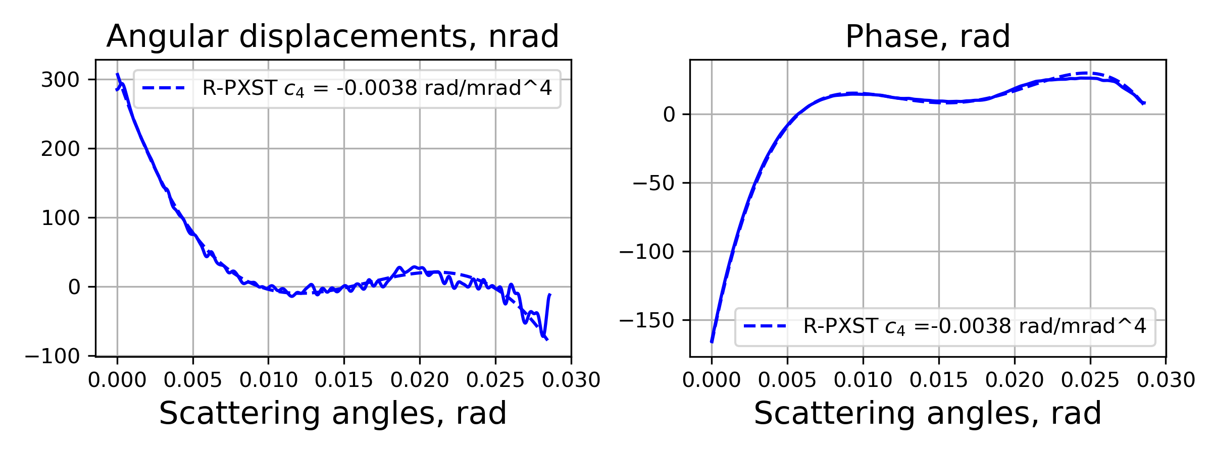
>>> fit_obj = fit_obj.remove_linear_term()
>>> fit = fit_obj.fit(max_order=3)

>>> fig, axes = plt.subplots(1, 2, figsize=(8, 3))
>>> axes[0].plot(fit_obj.thetas, fit_obj.theta_ab * 1e9, 'b')
>>> axes[0].plot(fit_obj.thetas, fit_obj.model(fit['fit']) * fit_obj.ref_ap * 1e9,
>>>              'b--', label=fr"R-PXST $c_4$ = {fit['c_4']:.4f} rad/mrad^4")
>>> axes[0].set_title('Angular displacements, nrad', fontsize=15)
>>>
>>> axes[1].plot(fit_obj.thetas, fit_obj.phase, 'b')
>>> axes[1].plot(fit_obj.thetas, fit_obj.model(fit['ph_fit']), 'b--',
>>>              label=fr"R-PXST $c_4$ ={fit['c_4']:.4f} rad/mrad^4")
>>> axes[1].set_title('Phase, rad', fontsize=15)
>>> for ax in axes:
>>>     ax.legend(fontsize=10)
>>>     ax.tick_params(labelsize=10)
>>>     ax.set_xlabel('Scattering angles, rad', fontsize=15)
>>>     ax.grid(True)
>>> plt.show()
Saving the results#
pyrost.cxi_converter_sigray() passes only a file handler pyrost.CXIStore for the input file.
In order to be able to save the results, we need to create a file handler for the output file:
>>> out_file = rst.CXIStore('sigray.cxi', mode='a')
>>> data = data.update_output_file(out_file)
Now we can save the results to the output file. By default pyrost.STData.save() saves all the data stored
inside the container. The method offers three modes:
‘overwrite’ : Overwrite all the data stored already in the output file.
‘append’ : Append data to the already existing data in the file.
‘insert’ : Insert the data into the already existing data at the set of frame indices idxs.
>>> data.save(mode='overwrite')