Performing a multislice beam propagation#
Experimental parameters#
Before performing the simulation, you need to define the experimental
parameters. You can do it with pyrost.multislice.MSParams.
The ms_sim library has built-in default parameters, which can be
accessed with pyrost.multislice.MSParams.import_default().
Note
Full list of experimental parameters is written in Simulation parameters. All the spatial parameters are assumed to be in microns.
>>> import pyrost.multislice as ms_sim
>>> params = ms_sim.MSParams.import_default()
>>> params = params.replace(x_step=5e-5, z_step=5e-3, n_min=100, n_max=5000,
>>>                         focus=1.5e3, mll_sigma=5e-5, mll_wl=6.2e-5, wl=6.2e-5,
>>>                         x_max=30.0, mll_depth=5.0)
Multilayer Laue lens#
As a sample, we use a Multilayer Laue lens (MLL).
pyrost.multislice.MLL can generate the transmission
profile of the MLL following the zone plate condition.
Note
MLL is a volume diffractive element for the efficient focusing of X-rays. This diffractive optical element consists of alternating layers of two materials, with the thicknesses of each layer being set to fulfill the zone plate condition:
Initialize an pyrost.multislice.MLL object with the parameters
params as follows:
>>> mll = ms_sim.MLL.import_params(params)
Performing the simulation#
Now you’re able to initialize the pyrost.multislice.MSPropagator
propagator, which does the multislice propagation with
pyrost.multislice.MSPropagator.beam_propagate(). You can
perform the simulation as follows:
>>> ms_prgt = ms_sim.MSPropagator(params, mll)
>>> ms_prgt.beam_propagate()
Note
The results are saved into ms_prgt.beam_profile and ms_prgt.smp_profile attributes. See MSPropagator for the full list of attributes.
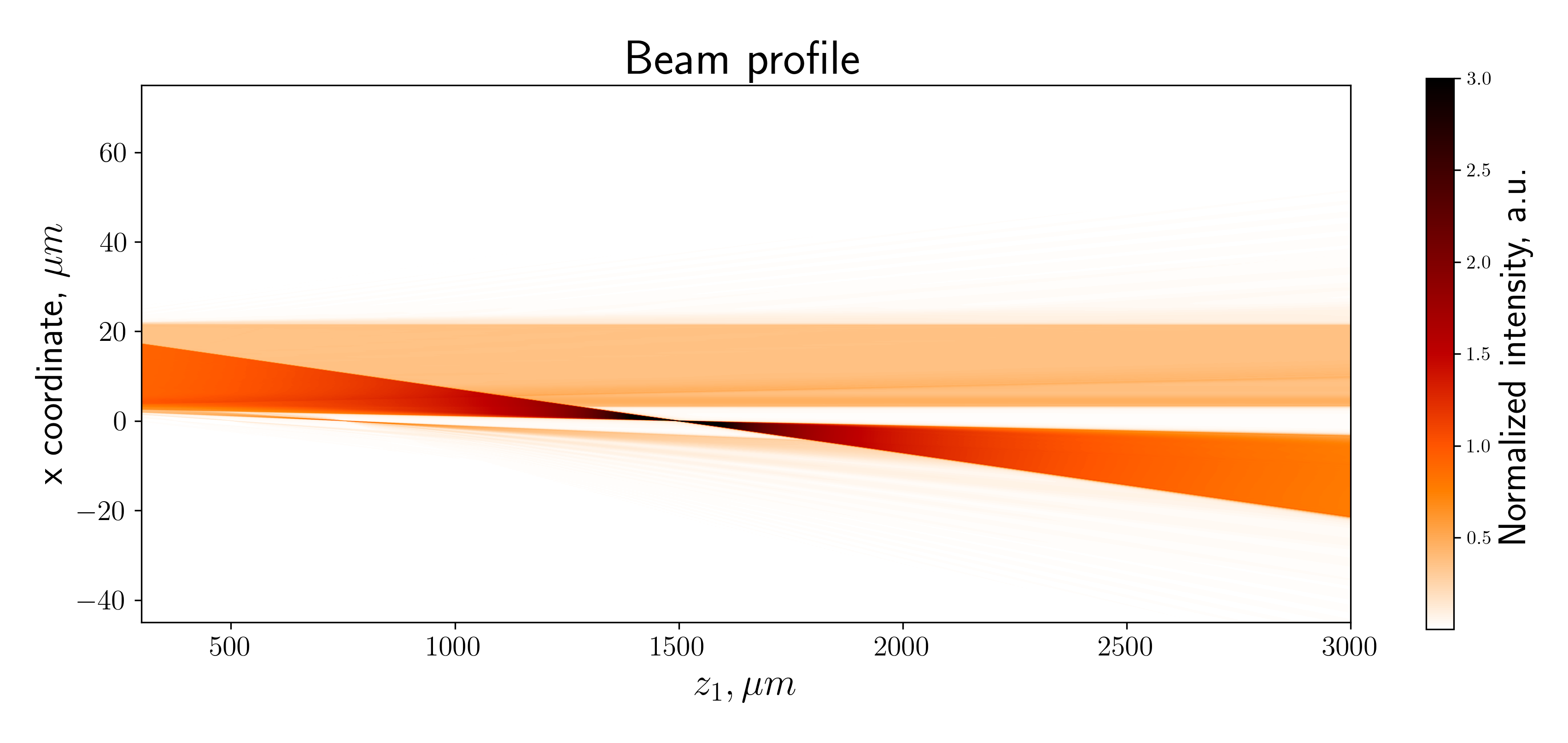
Whereupon you can generate the beam profile downstream of the sample, which is comprised of the direct beam and the convergent beam.
>>> z_arr = np.linspace(0.2 * params.focus, 2.0 * params.focus, 300)
>>> ds_beam, x_arr = ms_prgt.beam_downstream(z_arr, step=4.0 * params.x_step)

>>> fig, ax = plt.subplots(1, 1, figsize=(12, 6))
>>> im1 = ax.imshow(np.abs(ds_beam[::10]), vmax=3., cmap='gist_heat_r',
>>>                 extent=[z_arr.min(), z_arr.max(), x_arr.min(), x_arr.max()])
>>> cbar = fig.colorbar(im1, ax=ax, shrink=0.7)
>>> cbar.ax.set_ylabel('Normalized intensity, a.u.', fontsize=20)
>>> ax.set_ylabel(r'x coordinate, $\mu m$', fontsize=20)
>>> ax.set_aspect(10)
>>> ax.tick_params(labelsize=15)
>>> ax.set_xlabel(r'$z_1, \mu m$', fontsize=20)
>>> ax.set_title('Beam profile', fontsize=25)
>>> plt.show()