Speckle tracking reconstruction of a simulated dataset#

The speckle tracking update procedure of a one-dimensional scan doesn’t differ much from the case of a two-dimensional scan. See Speckle tracking reconstruction of a 2d dataset for an example.

1D scan CXI file#

To obtain the file generate it using Generating a speckle tracking dataset. The file has the following structure:

$ h5ls -r sim.cxi
/                        Group
/entry                   Group
/entry/data              Group
/entry/data/data         Dataset {200/Inf, 1, 985}
/entry/instrument        Group
/entry/instrument/detector Group
/entry/instrument/detector/distance Dataset {SCALAR}
/entry/instrument/detector/x_pixel_size Dataset {SCALAR}
/entry/instrument/detector/y_pixel_size Dataset {SCALAR}
/entry/instrument/source Group
/entry/instrument/source/wavelength Dataset {SCALAR}
/speckle_tracking        Group
/speckle_tracking/basis_vectors Dataset {200/Inf, 2, 3}
/speckle_tracking/defocus_x Dataset {SCALAR}
/speckle_tracking/defocus_y Dataset {SCALAR}
/speckle_tracking/mask   Dataset {200/Inf, 1, 985}
/speckle_tracking/pixel_translations Dataset {200/Inf, 2}
/speckle_tracking/translations Dataset {200/Inf, 3}
/speckle_tracking/whitefield Dataset {1, 985}

The file contains a ptychograph (set of frames summed over one of the detector axes) of 200 frames.

Loading the file#

The procedure for loading the data from a file is the same as in Speckle tracking reconstruction of a 2d dataset:

Create a pyrost.CXIProtocol protocol.
Open the input file with pyrost.CXIStore file handler. Create an output file. In this case, the output file is the same as the input one.
Create a pyrost.STData R-PXST data container.
Load all the data from the file with pyrost.STData.load().

>>> import pyrost as rst
>>> protocol = rst.CXIProtocol.import_default()
>>> inp_file = rst.CXIStore('sim.cxi', protocol=protocol)
>>> out_file = rst.CXIStore('sim.cxi', mode='a', protocol=protocol)
>>> data = rst.STData(input_file=inp_file, output_file=out_file)
>>> data = data.load()

The file already contains all the necessary attributes to perform the speckle tracking reconstruction:

>>> data.contents()
['whitefield', 'x_pixel_size', 'files', 'y_pixel_size', 'data', 'num_threads',
 'distance', 'defocus_x', 'good_frames', 'defocus_y', 'basis_vectors', 'translations',
 'mask', 'frames', 'wavelength', 'pixel_translations']

Speckle tracking update#

The steps to perform the speckle tracking update are also the same as in Speckle tracking update:

Create a pyrost.SpeckleTracking object.
Find an optimal kernel bandwidth with pyrost.SpeckleTracking.find_hopt().
Perform the iterative R-PXST update with pyrost.SpeckleTracking.train() or pyrost.SpeckleTracking.train_adapt().

>>> st_obj = data.get_st()
>>> h0 = st_obj.find_hopt()
>>> st_res = st_obj.train_adapt(search_window=(0.0, 10.0, 0.1), h0=h0, blur=8.0)

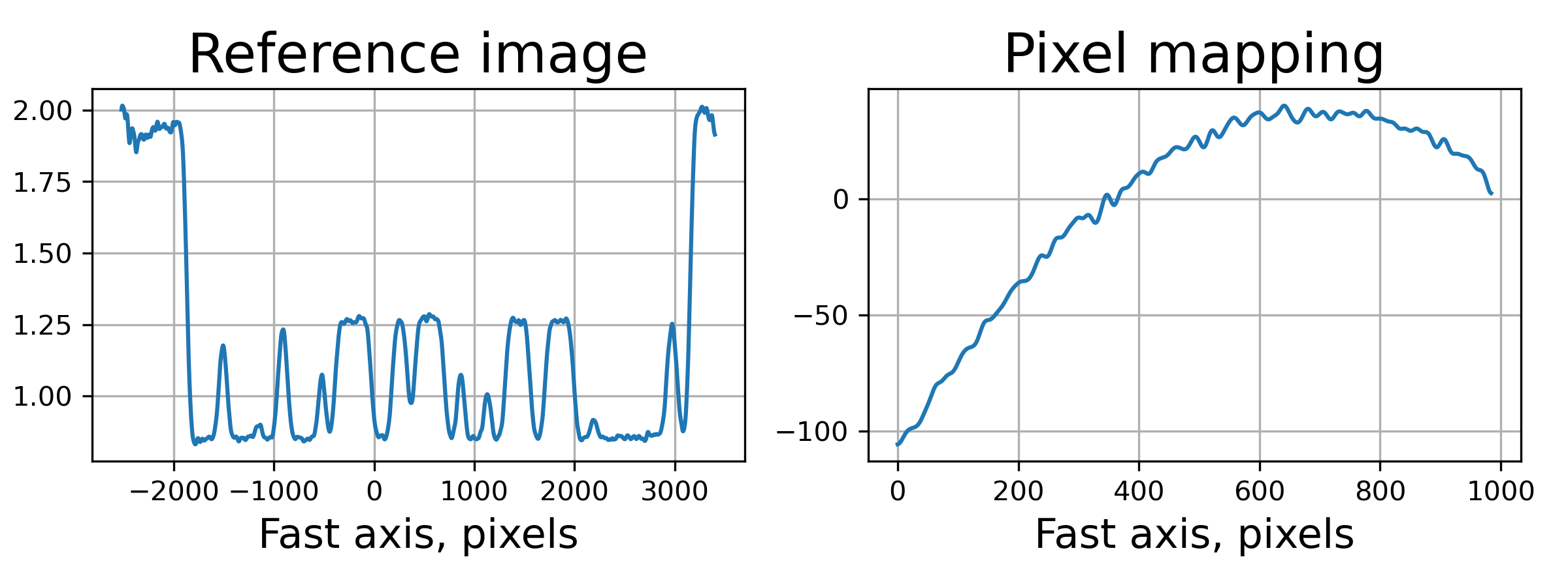
>>> fig, axes = plt.subplots(1, 2, figsize=(8, 3))
>>> axes[0].plot(np.arange(st_res.reference_image.shape[1]) - st_res.ref_orig[1],
>>>              st_res.reference_image[0])
>>> axes[0].set_title('Reference image', fontsize=20)
>>> axes[1].plot((st_res.pixel_map - st_obj.pixel_map)[1, 0])
>>> axes[1].set_title('Pixel mapping', fontsize=20)
>>> for ax in axes:
>>>     ax.tick_params(labelsize=15)
>>>     ax.set_xlabel('Fast axis, pixels', fontsize=15)
>>>     ax.grid(True)
>>> plt.show()

After we successfully reconstructed the wavefront with pyrost.SpeckleTracking.train_adapt() we are able to update the pyrost.STData container with pyrost.STData.import_st() method.

>>> data.import_st(st_res)

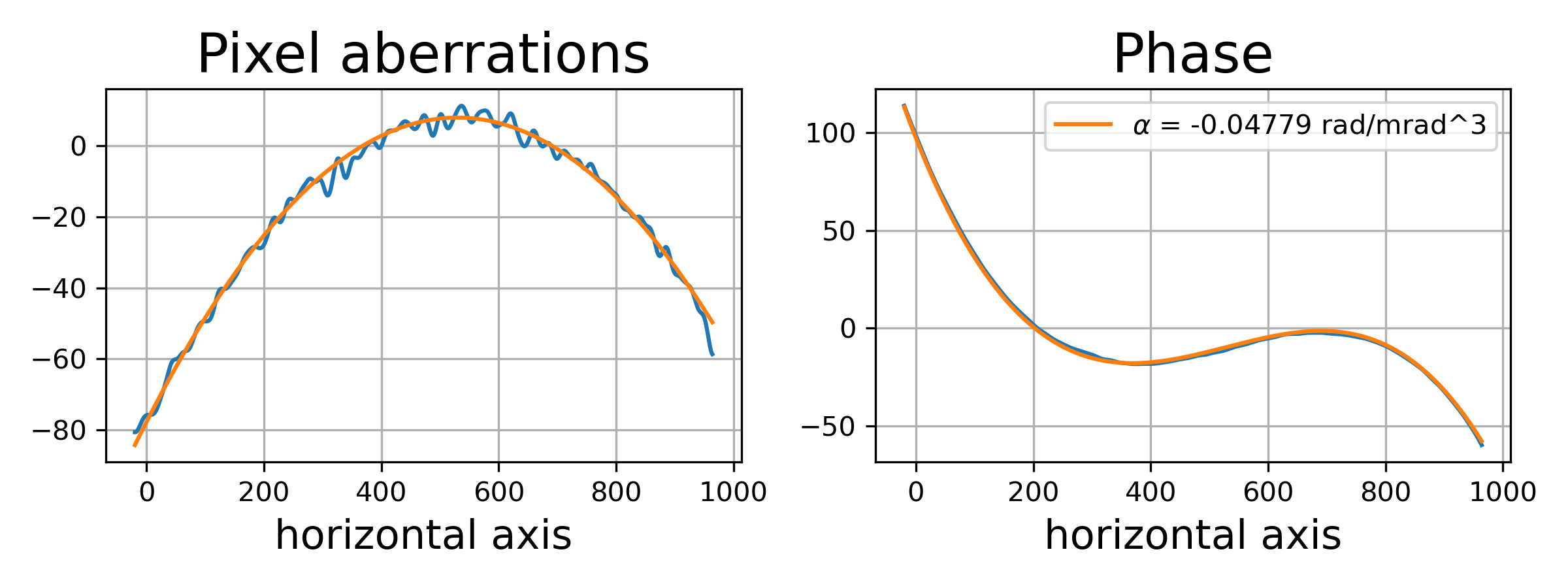
Phase reconstruction#

In the end, we want to look at an angular displacement profile of the X-ray beam and find the fit to the profile with a polynomial. All of it could be done with pyrost.AberrationsFit fitter object, which can be obtained with pyrost.STData.get_fit() method. We may parse the direct beam coordinate in pixels to center the scattering angles around the direction of the direct beam:

>>> fit_obj = data.get_fit(axis=1, center=20)

Moreover, we would like to remove the first-order polynomial term from the displacement profile with the pyrost.AberrationsFit.remove_linear_term(), since it characterizes the beam defocus and is of no interest to us. After that, you can obtain the best fit to the displacement profile with pyrost.AberrationsFit.fit() and to the phase profile with pyrost.AberrationsFit.fit_phase():

>>> fit_obj = fit_obj.remove_linear_term()
>>> fit = fit_obj.fit(max_order=2)
>>> print(fit['c_3'])
-0.04798021776009187

>>> fig, axes = plt.subplots(1, 2, figsize=(8, 3))
>>> axes[0].plot(fit_obj.pixels, fit_obj.pixel_aberrations)
>>> axes[0].plot(fit_obj.pixels, fit_obj.model(fit['fit']))
>>> axes[0].set_title('Pixel aberrations', fontsize=20)
>>> axes[1].plot(fit_obj.pixels, fit_obj.phase)
>>> axes[1].plot(fit_obj.pixels, fit_obj.model(fit['ph_fit']),
>>>              label=r'$\alpha$ = {:.5f} rad/mrad^3'.format(fit['c_3']))
>>> axes[1].set_title('Phase', fontsize=20)
>>> axes[1].legend(fontsize=10)
>>> for ax in axes:
>>>     ax.tick_params(axis='both', which='major', labelsize=15)
>>>     ax.set_xlabel('horizontal axis', fontsize=15)
>>> plt.tight_layout()
>>> plt.show()

Saving the results#

In the end, one can save the results to a CXI file. By default pyrost.STData.save() saves all the data it contains. The method offers three modes:

‘overwrite’ : Overwrite all the data stored already in the output file.
‘append’ : Append data to the already existing data in the file.
‘insert’ : Insert the data into the already existing data at the set of frame indices idxs.

>>> data.save(mode='overwrite')

$   h5ls -r results/sim_results/data_proc.cxi
/                        Group
/entry                   Group
/entry/data              Group
/entry/data/data         Dataset {200/Inf, 1, 985}
/entry/instrument        Group
/entry/instrument/detector Group
/entry/instrument/detector/distance Dataset {SCALAR}
/entry/instrument/detector/x_pixel_size Dataset {SCALAR}
/entry/instrument/detector/y_pixel_size Dataset {SCALAR}
/entry/instrument/source Group
/entry/instrument/source/wavelength Dataset {SCALAR}
/speckle_tracking        Group
/speckle_tracking/basis_vectors Dataset {200/Inf, 2, 3}
/speckle_tracking/defocus_x Dataset {SCALAR}
/speckle_tracking/defocus_y Dataset {SCALAR}
/speckle_tracking/mask   Dataset {200/Inf, 1, 985}
/speckle_tracking/phase  Dataset {1, 985}
/speckle_tracking/pixel_aberrations Dataset {2, 1, 985}
/speckle_tracking/pixel_translations Dataset {200/Inf, 2}
/speckle_tracking/reference_image Dataset {1, 5924}
/speckle_tracking/scale_map Dataset {1, 985}
/speckle_tracking/translations Dataset {200/Inf, 3}
/speckle_tracking/whitefield Dataset {1, 985}