Speckle tracking reconstruction of a 2d dataset#

Diatom dataset CXI file#

First, download the diatom.cxi file from the CXIDB. The file has the following structure:

$ h5ls -r diatom.cxi
/                        Group
/entry_1                 Group
/entry_1/data_1          Group
/entry_1/data_1/data     Dataset {121, 516, 1556}
/entry_1/data_1/experiment_identifier Dataset {121}
/entry_1/end_time        Dataset {SCALAR}
/entry_1/experiment_identifier Dataset, same as /entry_1/data_1/experiment_identifier
/entry_1/instrument_1    Group
/entry_1/instrument_1/detector_1 Group
/entry_1/instrument_1/detector_1/basis_vectors Dataset {121, 2, 3}
/entry_1/instrument_1/detector_1/corner_positions Dataset {121, 3}
/entry_1/instrument_1/detector_1/count_time Dataset {121, 1}
/entry_1/instrument_1/detector_1/data Dataset, same as /entry_1/data_1/data
/entry_1/instrument_1/detector_1/distance Dataset {SCALAR}
/entry_1/instrument_1/detector_1/experiment_identifier Dataset, same as /entry_1/data_1/experiment_identifier
/entry_1/instrument_1/detector_1/mask Dataset {516, 1556}
/entry_1/instrument_1/detector_1/name Dataset {SCALAR}
/entry_1/instrument_1/detector_1/x_pixel_size Dataset {SCALAR}
/entry_1/instrument_1/detector_1/y_pixel_size Dataset {SCALAR}
/entry_1/instrument_1/name Dataset {SCALAR}
/entry_1/instrument_1/source_1 Group
/entry_1/instrument_1/source_1/energy Dataset {SCALAR}
/entry_1/instrument_1/source_1/name Dataset {SCALAR}
/entry_1/instrument_1/source_1/wavelength Dataset {SCALAR}
/entry_1/sample_1        Group
/entry_1/sample_1/geometry Group
/entry_1/sample_1/geometry/orientation Dataset {121, 6}
/entry_1/sample_1/geometry/translation Dataset {121, 3}
/entry_1/sample_1/name   Dataset {SCALAR}
/entry_1/start_time      Dataset {SCALAR}

As we can see in entry_1/data_1/data, the file contains a two-dimensional 11x11 scan, where each frame is an image of 516x1556 pixels.

Loading the data#

CXI protocol#

Before loading the file, a CXI protocol for the file diatom.cxi must be created (see pyrost.CXIProtocol for more information). The CXI protocol must be instantiated with the following information for all the data attributes (data, whitefield, etc.) needed for PXST data processing:

datatypes : Data type of the given data attribute.
load_paths : Lost of the paths inside a CXI file, where the given data attribute may be saved.
kind : A kind of the data array of the given attribute (see pyrost.CXIProtocol for more information).

pyrost offers a default CXI protocol via pyrost.CXIProtocol.import_default(), that contains all the necessary data for the diatom.cxi file:

>>> import pyrost as rst
>>> import numpy as np
>>> protocol = rst.CXIProtocol.import_default()

CXI file handler#

pyrost.CXIStore is a file handler object, it accepts a pyrost.CXIProtocol protocol and paths to a single file or a set of files. It reads the files for all the data attributes specified in the procotol. The file handler provides two methods to load and save the data for the specified data attribute (pyrost.CXIStore.load_attribute() and pyrost.CXIStore.save_attribute()).

Read diatom.cxi file as follows: .. doctest:

>>> inp_file = rst.CXIStore('diatom.cxi', protocol=protocol)

We will save the results to a diatom_proc.cxi file: .. doctest:

>>> out_file = rst.CXIStore('results/exp/diatom_proc.cxi', mode='a',
>>>                         protocol=protocol)

Preprocessing of a PXST dataset#

Now one may load the data from diatom.cxi file and generate the quantities needed prior to the main speckle tracking update procedure with a pyrost.STData data container. pyrost.STData need a pyrost.CXIStore file handler for an input file for the initialization. We also pass a file handler of the output file too (it’s optional, the output file handler can be updated with pyrost.STData.update_output_file()):

>>> data = rst.STData(input_file=inp_file, output_file=out_file)

pyrost.STData offers two methods to load the data to the container from the input files (pyrost.STData.load()) and save the data stored in the container to the output file (pyrost.STData.save()). Let’s load the data store in the diatom.cxi file:

>>> data = data.load(processes=4)

In order to conduct image transforms on the measured frames, pyrost offers a set of image transforms (pyrost.Mirror, pyrost.Crop, pyrost.Downscale), that can be passed to the container:

>>> crop = rst.Crop(roi=[80, 420, 60, 450])
>>> data = data.update_transform(transform=crop)

pyrost.STData contains a set of data processing tools to work with the data. In particular, pyrost.STData.update_mask() generates a pixel mask that excludes bad and hot pixels of the dataset from the subsequent analysis, pyrost.STData.mask_frames() selects the good frames that will be used in the speckle tracking reconstruction:

>>> data = data.update_mask(method='perc-bad')
>>> data = data.mask_frames(good_frames=np.arange(1, 121))

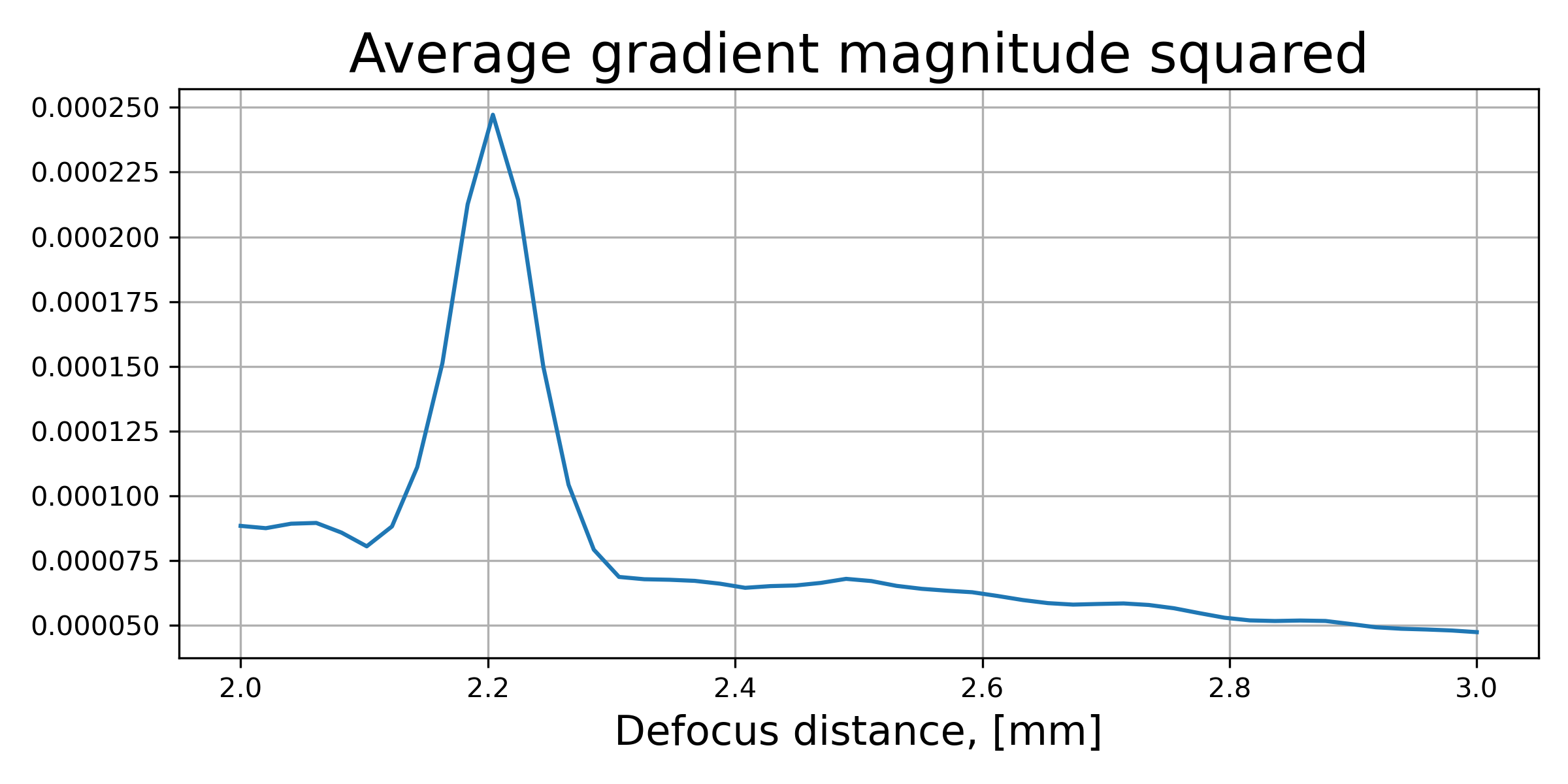
Now we need to estimate the defocus distance needed for the R-PXST update procedure. One can estimate it with pyrost.STData.defocus_sweep(). It generates reference images for a set of defocus distances and yields average values of the gradient magnitude squared (\(\left< R[i, j] \right>\), see pyrost.STData.defocus_sweep()), which serves a figure of merit of how sharp or blurry the reference image is (the higher is \(\left< R[i, j] \right>\) the sharper is the reference profile).

>>> defoci = np.linspace(2e-3, 3e-3, 50)
>>> sweep_scan = data.defocus_sweep(defoci, size=5, hval=1.5)
>>> defocus = defoci[np.argmax(sweep_scan)]
>>> print(defocus)
0.002204081632653061

>>> fig, ax = plt.subplots(figsize=(8, 4))
>>> ax.plot(defoci * 1e3, sweep_scan)
>>> ax.set_xlabel('Defocus distance, [mm]', fontsize=20)
>>> ax.set_title('Average gradient magnitude squared', fontsize=20)
>>> ax.tick_params(labelsize=15)
>>> ax.grid(True)
>>> plt.show()

Let’s update the data container with the defocus distance we’ve got.

>>> data = data.update_defocus(defocus)

Speckle tracking update#

Creating a `SpeckleTracking` object#

Having formed an initial estimate for the defocus distance and the white-field (or a set of white-fields, if needed), a pyrost.SpeckleTracking object with all data attributes necessary for the R-PXST update can be generated. The key attributes that it contains are:

reference_image : Unaberrated reference profile of the sample.
pixel_map : Discrete geometrical mapping function from the detector plane to the reference plane.
data : Stack of measured frames.
whitefield : White-field of the measured holograms (frames).
di_pix, dj_pix : Vectors of sample translations converted to pixels along the vertical and horizontal axes, respectively.

Iterative R-PXST reconstruction#

pyrost.SpeckleTracking provides an interface to refine the reference image and lens wavefront iteratively. It offers two methods to choose from:

pyrost.SpeckleTracking.train() : performs the iterative reference image and pixel mapping updates with the constant kernel bandwidths for the reference image estimator (h0).
pyrost.SpeckleTracking.train_adapt() : does ditto, but updates the bandwidth value for the reference image estimator at each iteration by the help of the BFGS method to attain the minimum error value.

Note

You should pay outmost attention to choosing the right kernel bandwidth of the reference image estimator (h0 in pyrost.SpeckleTracking.update_reference()). Essentially it stands for the high frequency cut-off imposed during the reference profile update, so it helps to supress the noise. If the value is too high, you’ll lose useful information in the reference profile. If the value is too low and the data is noisy, you won’t get an accurate reconstruction. An optimal kernel bandwidth can be estimated with pyrost.SpeckleTracking.find_hopt() method.

Note

Next important parameter is blur in pyrost.SpeckleTracking.update_pixel_map(). It helps to prevent noise propagation to the next iteration by means of kernel smoothing of the updated pixel mapping.

Note

Apart from pixel mapping update, one may try to perform the sample shifts update if you’ve got a low precision or credibility of sample shifts measurements. It can be done by setting the update_translations parameter to True.

Optimal kernel bandwidth#

Kernel bandwidth is an important hyperparameter in the reference image update. Using a small kernel bandwidth in a non-parametric estimator can introduce a small bias to the estimate. At the same time, less smoothing means that each estimate is obtained by averaging over (in effect) just a few observations, making the estimate noisier. So less smoothing increases the variance of the estimate. Our implementation estimates the optimal bandwidth based on minimizing the cross-validation metric. pyrost.SpeckleTracking divides the dataset into two subsets at the initialization stage. The splitting into two subsets can be updated with pyrost.SpeckleTracking.test_train_split():

>>> st_obj = data.get_st(ds_x=1.0, ds_y=1.0)
>>> st_obj = st_obj.test_train_split(test_ratio=0.2)

The CV method calculates the CV as follows: it generates a reference profile based on the former “training” subset and calculates the mean-squared-error for the latter “testing” subset. The CV can be calculated with pyrost.SpeckleTracking.CV() and pyrost.SpeckleTracking.CV_curve():

>>> h_vals = np.linspace(0.5, 3.0, 25)
>>> cv_vals = st_obj.CV_curve(h_vals)

>>> fig, ax = plt.subplots(figsize=(8, 4))
>>> ax.plot(h_vals, cv_vals)
>>> ax.set_xlabel('Kernel bandwidth', fontsize=15)
>>> ax.set_title('Cross-validation', fontsize=20)
>>> ax.tick_params(labelsize=10)
>>> ax.grid(True)
>>> plt.show()

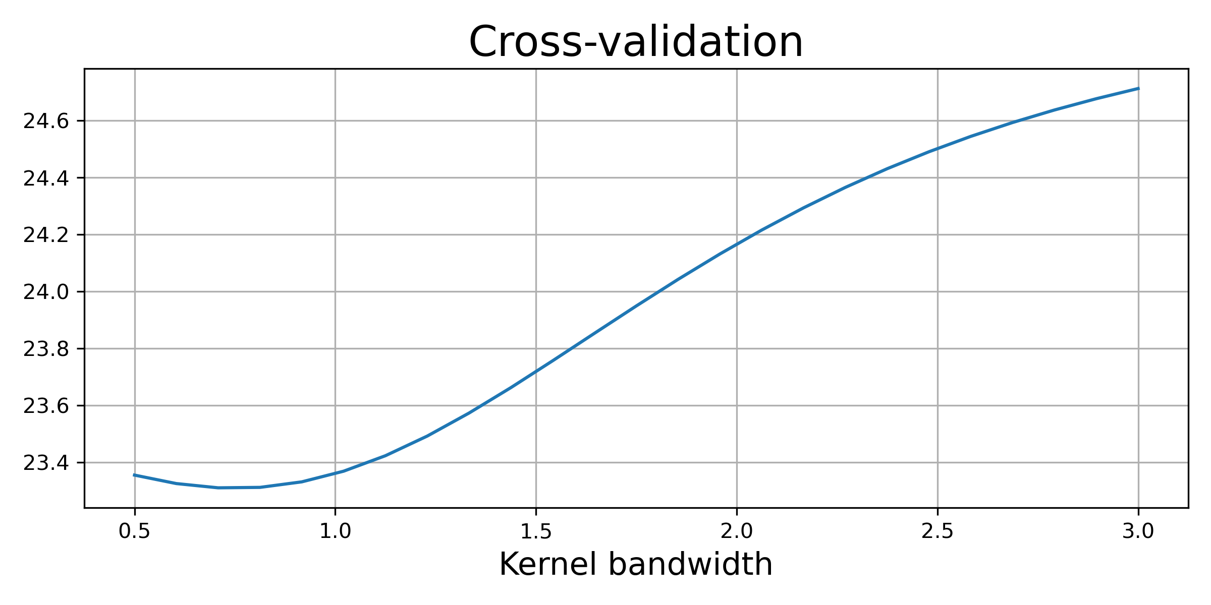
The optimal kernel bandwidth can be estimated by finding a minimum of CV with the quasi-Newton method of Broyden, Fletcher, Goldfarb, and Shanno [BFGS]:

>>> h0 = st_obj.find_hopt(verbose=True)
>>> print(h0)
0.7537624318448054

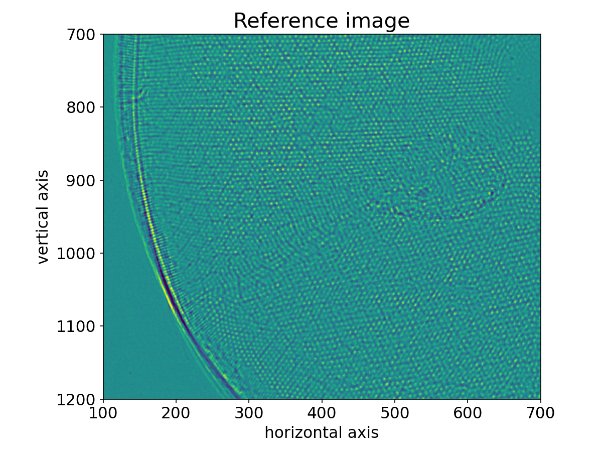
Performing the iterative R-PXST update#

Now having an estimate of the optimal kernel bandwidth, we’re ready to perform an iterative update with pyrost.SpeckleTracking.train_adapt():

>>> st_res = st_obj.train_adapt(search_window=(5.0, 5.0, 0.1), h0=h0, blur=8.0, n_iter=10,
>>>                             pm_method='rsearch', pm_args={'n_trials': 50})

The results are saved to a st_res container:

>>> fig, ax = plt.subplots(figsize=(8, 6))
>>> ax.imshow(st_res.reference_image[700:1200, 100:700], vmin=0.7, vmax=1.3,
>>>           extent=[100, 700, 1200, 700])
>>> ax.set_title('Reference image', fontsize=20)
>>> ax.set_xlabel('horizontal axis', fontsize=15)
>>> ax.set_ylabel('vertical axis', fontsize=15)
>>> ax.tick_params(labelsize=15)
>>> plt.show()

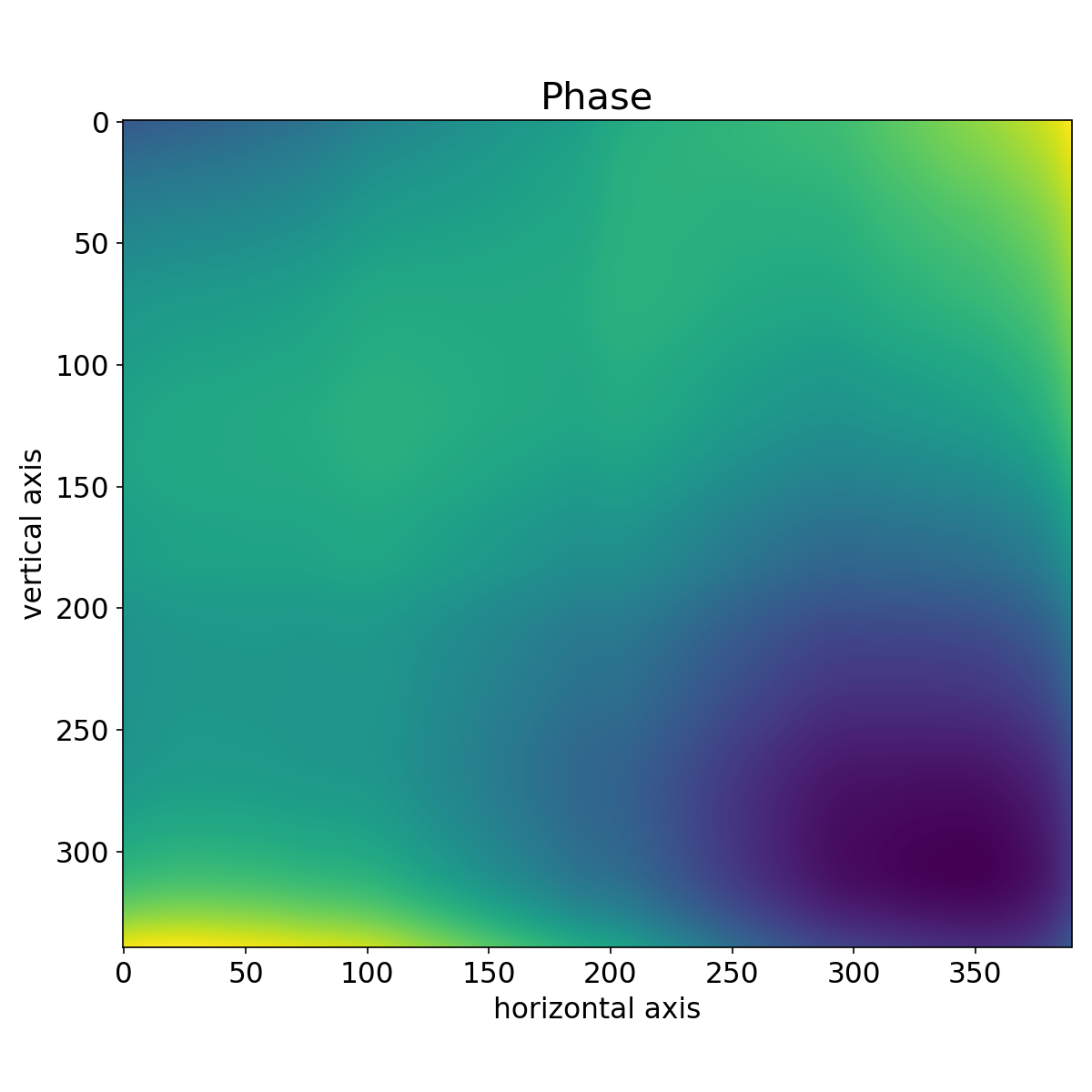
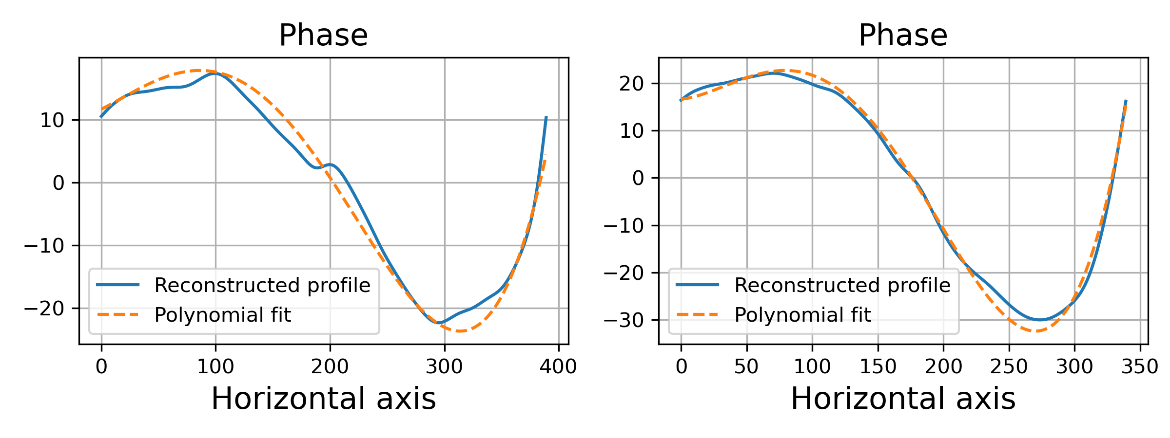
Phase reconstruction#

We got the pixel mapping from the detector plane to the reference plane, which can be easily translated to the angular displacement profile of the lens. Following the Hartmann sensor principle (look [ST] page 762 for more information), we reconstruct the lens’ phase profile with pyrost.STData.import_st() method. Besides, one can fit the phase profile with a polynomial function using pyrost.AberrationsFit fitter object, which can be obtained with pyrost.STData.get_fit() method.

>>> data.import_st(st_res)
>>> fit_obj_ss = data.get_fit(axis=0)
>>> fit_ss = fit_obj_ss.fit(max_order=3)
>>> fit_obj_fs = data.get_fit(axis=1)
>>> fit_fs = fit_obj_fs.fit(max_order=3)

>>> fig, ax = plt.subplots(figsize=(8, 8))
>>> ax.imshow(data.get('phase'))
>>> ax.set_title('Phase', fontsize=20)
>>> ax.set_xlabel('Horizontal axis', fontsize=15)
>>> ax.set_ylabel('Vertical axis', fontsize=15)
>>> ax.tick_params(labelsize=15)
>>> plt.show()

>>> fig, axes = plt.subplots(1, 2, figsize=(8, 3))
>>> axes[0].plot(fit_obj_fs.pixels, fit_obj_fs.phase, label='Reconstructed profile')
>>> axes[0].plot(fit_obj_fs.pixels, fit_obj_fs.model(fit_fs['ph_fit']), linestyle='dashed',
                 label='Polynomial fit')
>>> axes[0].set_xlabel('Horizontal axis', fontsize=15)
>>> axes[1].plot(fit_obj_ss.pixels, fit_obj_ss.phase, label='Reconstructed profile')
>>> axes[1].plot(fit_obj_ss.pixels, fit_obj_ss.model(fit_ss['ph_fit']), linestyle='dashed',
>>>              label='Polynomial fit')
>>> axes[1].set_xlabel('Horizontal axis', fontsize=15)
>>> for ax in axes:
>>>     ax.set_title('Phase', fontsize=15)
>>>     ax.tick_params(labelsize=10)
>>>     ax.legend(fontsize=10)
>>>     ax.grid(True)
>>> plt.show()

Saving the results#

In the end, one can save the results to a CXI file. By default pyrost.STData.save() saves all the data it contains. The method offers three modes:

‘overwrite’ : Overwrite all the data stored already in the output file.
‘append’ : Append data to the already existing data in the file.
‘insert’ : Insert the data into the already existing data at the set of frame indices idxs.

>>> data.save(mode='overwrite')

To see all the attributes stored in the container, use pyrost.STData.contents():

>>> data.contents()
['translations', 'mask', 'phase', 'whitefield', 'num_threads', 'reference_image', 'distance',
'wavelength', 'pixel_aberrations', 'good_frames', 'x_pixel_size', 'files', 'y_pixel_size',
'scale_map', 'defocus_y', 'frames', 'pixel_translations', 'transform', 'data', 'basis_vectors',
'defocus_x']

Here are all the results saved in the output file diatom_proc.cxi:

$   h5ls -r diatom_proc.cxi
/                        Group
/entry                   Group
/entry/data              Group
/entry/data/data         Dataset {120/Inf, 340, 390}
/entry/instrument        Group
/entry/instrument/detector Group
/entry/instrument/detector/distance Dataset {SCALAR}
/entry/instrument/detector/x_pixel_size Dataset {SCALAR}
/entry/instrument/detector/y_pixel_size Dataset {SCALAR}
/entry/instrument/source Group
/entry/instrument/source/wavelength Dataset {SCALAR}
/speckle_tracking        Group
/speckle_tracking/basis_vectors Dataset {120/Inf, 2, 3}
/speckle_tracking/defocus_x Dataset {SCALAR}
/speckle_tracking/defocus_y Dataset {SCALAR}
/speckle_tracking/mask   Dataset {120/Inf, 340, 390}
/speckle_tracking/phase  Dataset {340, 390}
/speckle_tracking/pixel_aberrations Dataset {2, 340, 390}
/speckle_tracking/pixel_translations Dataset {120/Inf, 2}
/speckle_tracking/reference_image Dataset {1442, 1475}
/speckle_tracking/scale_map Dataset {340, 390}
/speckle_tracking/translations Dataset {120/Inf, 3}
/speckle_tracking/whitefield Dataset {340, 390}

As one can see, all the results have been saved using the same CXI protocol.

References#

ST: “Ptychographic X-ray speckle tracking”, Morgan, A. J., Quiney, H. M., Bajt, S. & Chapman, H. N. (2020). J. Appl. Cryst. 53, 760-780.

Speckle tracking reconstruction of a 2d dataset#

Diatom dataset CXI file#

Loading the data#

CXI protocol#

CXI file handler#

Preprocessing of a PXST dataset#

Speckle tracking update#

Creating a SpeckleTracking object#

Iterative R-PXST reconstruction#

Optimal kernel bandwidth#

Performing the iterative R-PXST update#

Phase reconstruction#

Saving the results#

References#

Creating a `SpeckleTracking` object#