Diatom
Diatom CXI File
First download the diatom.cxi file from the CXIDB. The file has the following structure:
$ h5ls -r results/diatom.cxi
/                        Group
/entry_1                 Group
/entry_1/data_1          Group
/entry_1/data_1/data     Dataset {121, 516, 1556}
/entry_1/data_1/experiment_identifier Dataset {121}
/entry_1/end_time        Dataset {SCALAR}
/entry_1/experiment_identifier Dataset, same as /entry_1/data_1/experiment_identifier
/entry_1/instrument_1    Group
/entry_1/instrument_1/detector_1 Group
/entry_1/instrument_1/detector_1/basis_vectors Dataset {121, 2, 3}
/entry_1/instrument_1/detector_1/corner_positions Dataset {121, 3}
/entry_1/instrument_1/detector_1/count_time Dataset {121, 1}
/entry_1/instrument_1/detector_1/data Dataset, same as /entry_1/data_1/data
/entry_1/instrument_1/detector_1/distance Dataset {SCALAR}
/entry_1/instrument_1/detector_1/experiment_identifier Dataset, same as /entry_1/data_1/experiment_identifier
/entry_1/instrument_1/detector_1/mask Dataset {516, 1556}
/entry_1/instrument_1/detector_1/name Dataset {SCALAR}
/entry_1/instrument_1/detector_1/x_pixel_size Dataset {SCALAR}
/entry_1/instrument_1/detector_1/y_pixel_size Dataset {SCALAR}
/entry_1/instrument_1/name Dataset {SCALAR}
/entry_1/instrument_1/source_1 Group
/entry_1/instrument_1/source_1/energy Dataset {SCALAR}
/entry_1/instrument_1/source_1/name Dataset {SCALAR}
/entry_1/instrument_1/source_1/wavelength Dataset {SCALAR}
/entry_1/sample_1        Group
/entry_1/sample_1/geometry Group
/entry_1/sample_1/geometry/orientation Dataset {121, 6}
/entry_1/sample_1/geometry/translation Dataset {121, 3}
/entry_1/sample_1/name   Dataset {SCALAR}
/entry_1/start_time      Dataset {SCALAR}
As we can see in entry_1/data_1/data the file contains a two-dimensional 11x11 scan,
where each frame is an image of 516x1556 pixels.
Loading the file
Load the CXI file into a data container pyrost.STData with pyrost.STLoader.
pyrost.loader() returns the default loader with the default CXI protocol
(pyrost.protocol()).
Note
pyrost.STLoader will raise an AttributeError while loading the data
from the CXI file if some of the necessary attributes for Speckle Tracking algorithm
are not provided. You can see full list of the necessary attributes in
pyrost.STData. Adding the missing attributes to pyrost.STLoader.load()
solves the problem.
>>> import pyrost as rst
>>> loader = rst.loader()
>>> data = loader.load('results/diatom.cxi')
Moreover, you can crop the data with the provided region of interest at the detector plane,
or mask bad frames and bad pixels (See pyrost.STData.crop_data(),
pyrost.STData.mask_frames(), pyrost.STData.make_mask()).
>>> data = loader.load('results/diatom.cxi', roi=(75, 420, 55, 455), good_frames=np.arange(1, 121))
>>> data = data.make_mask(method='perc-bad')
OR
>>> data = data.crop_data(roi=(75, 420, 55, 455))
>>> data = data.mask_frames(good_frames=np.arange(1, 121))
>>> data = data.make_mask(method='perc-bad')
It worked! But still we can not perform the Speckle Tracking update procedure without the
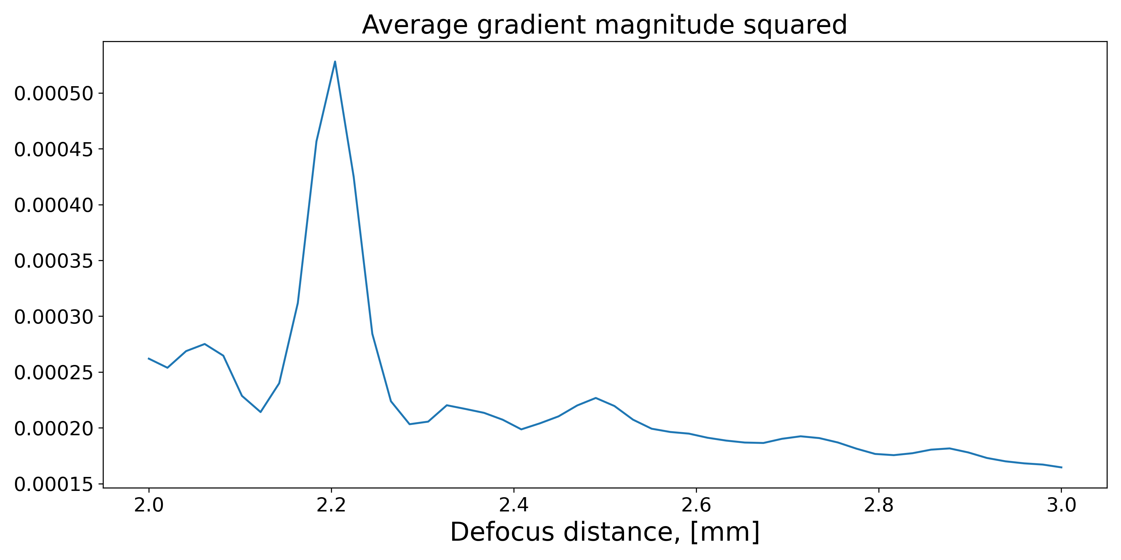
estimates of the defocus distance. You can estimate it with pyrost.STData.defocus_sweep().
It generates sample profiles for the set of defocus distances and yields an average value
of gradient magnitude squared (\(\left| \nabla I_{ref} \right|^2\)), which characterizes
reference image’s contrast (the higher the value the better the estimate of defocus distance
is).
>>> defoci = np.linspace(2e-3, 3e-3, 50)
>>> sweep_scan = data.defocus_sweep(defoci, ls_ri=0.7)
>>> defocus = defoci[np.argmax(sweep_scan)]
>>> print(defocus)
0.002204081632653061

>>> fig, ax = plt.subplots(figsize=(12, 6))
>>> ax.plot(defoci * 1e3, sweep_scan)
>>> ax.set_xlabel('Defocus distance, [mm]', fontsize=20)
>>> ax.set_title('Average gradient magnitude squared', fontsize=20)
>>> ax.tick_params(labelsize=15)
>>> plt.show()
Let’s update the data container with the defocus distance we got.
>>> data = data.update_defocus(defocus)
Speckle Tracking update
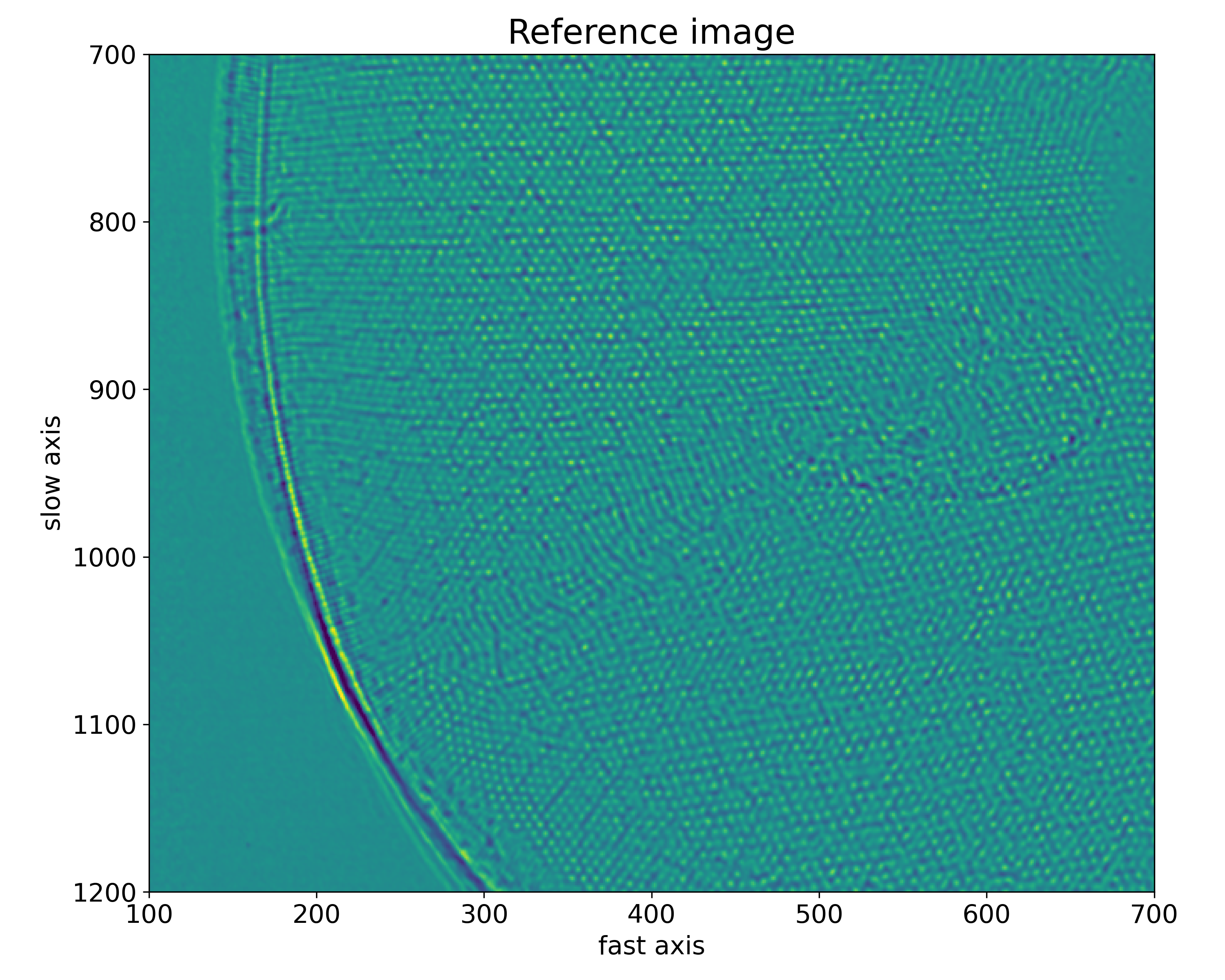
Now we’re ready to generate a pyrost.SpeckleTracking object, which does the heavy
lifting of calculating the pixel mapping between reference plane and detector’s plane,
and generating the unabberated profile of the sample.
Note
You should pay outmost attention to choose the right length scales of reference image and pixel mapping (ls_ri, ls_pm). Essentually they stand for high frequency cut-off of the measured data, it helps to supress Poisson noise. If the values are too high you’ll lose useful information. If the values are too low in presence of high noise, you won’t get accurate results.
Note
Apart from pixel mapping update you may try to perform sample shifts update if you’ve
got low precision or credibilily of sample shifts measurements. You can do it with pyrost.SpeckleTracking.iter_update()
if you assign True to update_translations argument.
>>> st_obj = data.get_st()
>>> st_res, errors = st_obj.iter_update(sw_fs=15, sw_ss=15, ls_pm=1.5, ls_ri=0.7, verbose=True, n_iter=5)
Iteration No. 0: Total MSE = 0.798
Iteration No. 1: Total MSE = 0.711
Iteration No. 2: Total MSE = 0.256
Iteration No. 3: Total MSE = 0.205
Iteration No. 4: Total MSE = 0.209

>>> fig, ax = plt.subplots(figsize=(10, 10))
>>> ax.imshow(st_res.reference_image[700:1200, 100:700], vmin=0.7, vmax=1.3, extent=[100, 700, 1200, 700])
>>> ax.set_title('Reference image', fontsize=20)
>>> ax.set_xlabel('fast axis', fontsize=15)
>>> ax.set_ylabel('slow axis', fontsize=15)
>>> ax.tick_params(labelsize=15)
>>> plt.show()
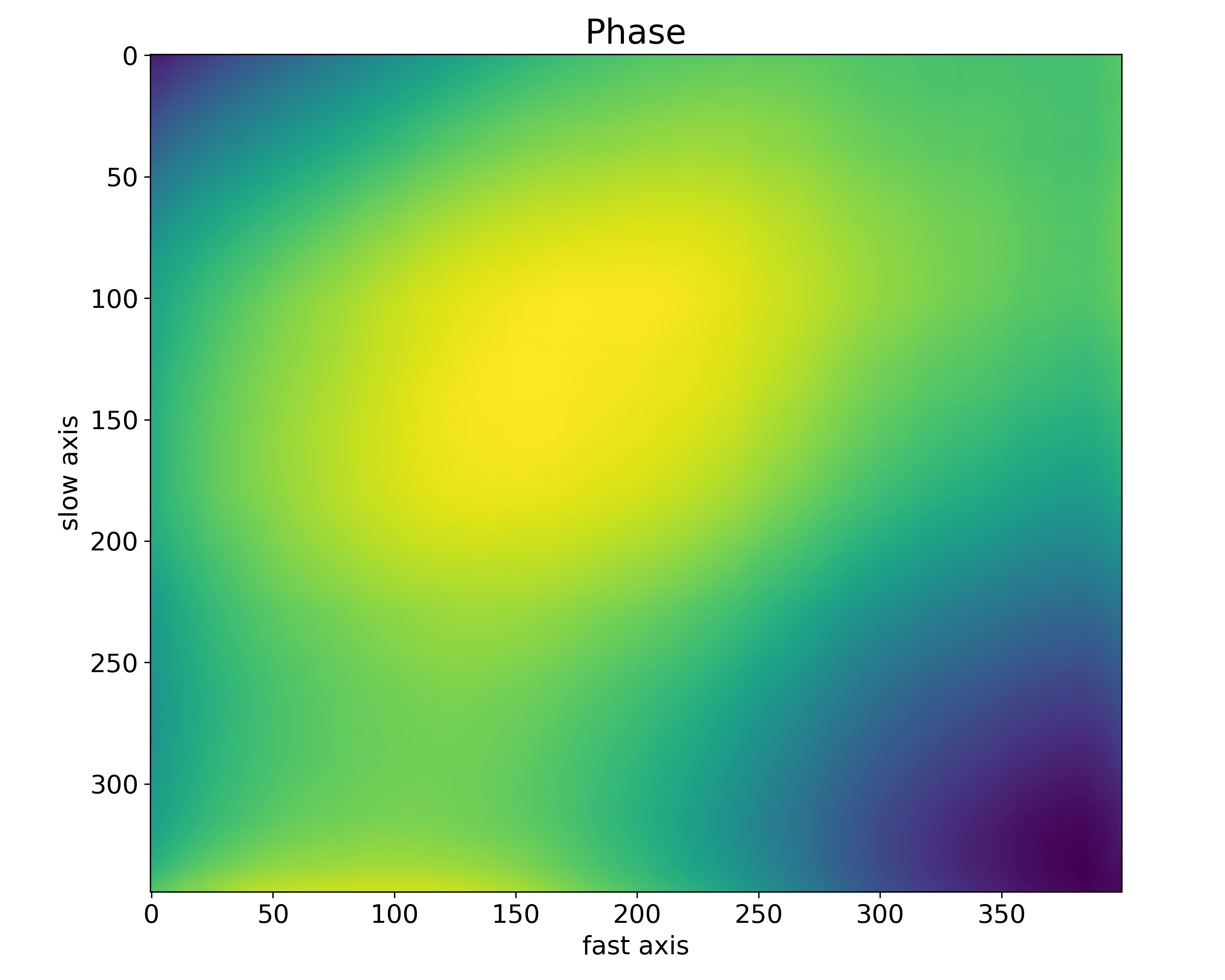
Phase reconstruction
We got the pixel map, which can be easily translated to the deviation angles of the lens
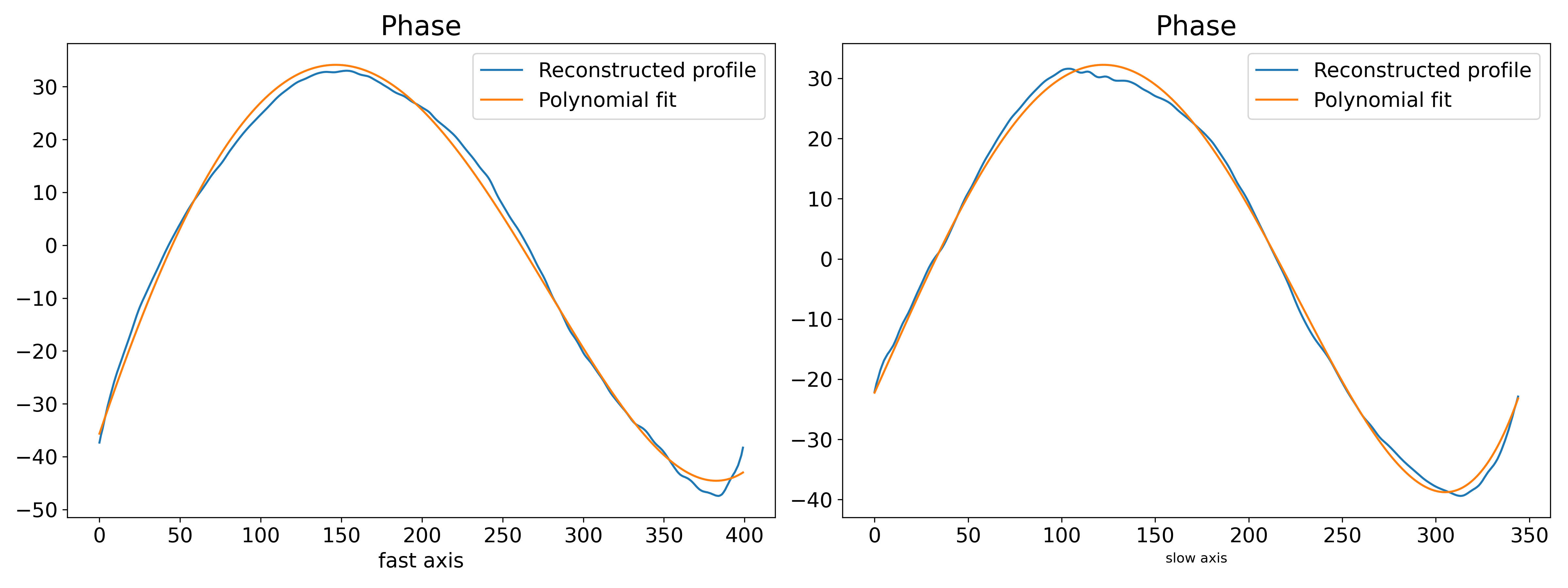
wavefront. Now we’re able to reconstruct the lens’ phase profile. Besides, you can fit
the phase profile with polynomial function using pyrost.AbberationsFit.
>>> data.update_phase(st_res)
>>> fit_obj_ss = data.get_fit(axis=0)
>>> fit_ss = fit_obj_ss.fit(max_order=3)
>>> fit_obj_fs = data.get_fit(axis=1)
>>> fit_fs = fit_obj_fs.fit(max_order=3)

>>> fig, ax = plt.subplots(figsize=(10, 10))
>>> ax.imshow(data.get('phase'))
>>> ax.set_title('Phase', fontsize=20)
>>> ax.set_xlabel('fast axis', fontsize=15)
>>> ax.set_ylabel('slow axis', fontsize=15)
>>> ax.tick_params(labelsize=15)
>>> plt.show()
>>> fig, axes = plt.subplots(1, 2, figsize=(16, 6))
>>> axes[0].plot(fit_obj_fs.pixels, fit_obj_fs.phase, label='Reconstructed profile')
>>> axes[0].plot(fit_obj_fs.pixels, fit_obj_fs.model(fit_fs['ph_fit']),
                 label='Polynomial fit')
>>> axes[0].set_xlabel('fast axis', fontsize=15)
>>> axes[1].plot(fit_obj_ss.pixels, fit_obj_ss.phase, label='Reconstructed profile')
>>> axes[1].plot(fit_obj_ss.pixels, fit_obj_ss.model(fit_ss['ph_fit']),
>>>              label='Polynomial fit')
>>> axes[1].set_xlabel('slow axis')
>>> for ax in axes:
>>>     ax.set_title('Phase', fontsize=20)
>>>     ax.tick_params(labelsize=15)
>>>     ax.legend(fontsize=15)
>>> plt.show()
Saving the results
In the end you can save the results to a CXI file.
>>> with h5py.File('results/diatom_proc.cxi', 'w') as cxi_file:
>>>     data.write_cxi(cxi_file)
$   h5ls -r diatom_proc.cxi
/                        Group
/entry_1                 Group
/entry_1/data_1          Group
/entry_1/data_1/data     Dataset {121, 516, 1556}
/entry_1/instrument_1    Group
/entry_1/instrument_1/detector_1 Group
/entry_1/instrument_1/detector_1/basis_vectors Dataset {121, 2, 3}
/entry_1/instrument_1/detector_1/distance Dataset {SCALAR}
/entry_1/instrument_1/detector_1/x_pixel_size Dataset {SCALAR}
/entry_1/instrument_1/detector_1/y_pixel_size Dataset {SCALAR}
/entry_1/instrument_1/source_1 Group
/entry_1/instrument_1/source_1/wavelength Dataset {SCALAR}
/entry_1/sample_1        Group
/entry_1/sample_1/geometry Group
/entry_1/sample_1/geometry/translations Dataset {121, 3}
/frame_selector          Group
/frame_selector/good_frames Dataset {120}
/speckle_tracking        Group
/speckle_tracking/error_frame Dataset {516, 1556}
/speckle_tracking/dfs    Dataset {SCALAR}
/speckle_tracking/dss    Dataset {SCALAR}
/speckle_tracking/mask   Dataset {516, 1556}
/speckle_tracking/phase  Dataset {516, 1556}
/speckle_tracking/pixel_abberations Dataset {2, 516, 1556}
/speckle_tracking/pixel_map Dataset {2, 516, 1556}
/speckle_tracking/pixel_translations Dataset {121, 2}
/speckle_tracking/reference_image Dataset {1455, 1498}
/speckle_tracking/roi    Dataset {4}
/speckle_tracking/whitefield Dataset {516, 1556}
As you can see all the results have been saved using the same CXI protocol.